Table of Contents
Project Statement and Goals
Motivation and Background
Data Description
EDA
Data Cleaning
Metrics
Model Training
Interpreting the Model
Model Testing and Results
Conclusion and What’s Next
Literature Review
Conclusion and What’s Next
Conclusion
We have far from cutting edge results, but we built a system that returns reasonable results and is close in r-precision to some teams on the Spotify MPD Competition site: see here.
We gained experience working with a large dataset in which observations are largely categorical text data. We have gleaned insight into what happens on Spotify servers when we load up this week’s ‘Your Discovered Weekly’ and hit play. More broadly, we have enaged with the inner workings of technology that for most people just works.
Expanding the Project’s Scope
Working with 1,000,000 Playlists
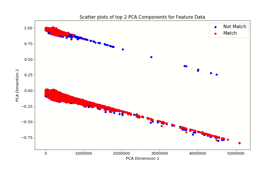
One idea we could use to better handle computing on the full dataset is principal component analysis. By narrowing down our set of features we could train models faster and experiment more with model tuning. We did create a visualization to see how we can differentiate between match = 0 and match = 1 tracks using the first 2 principal components. We can see that even just two components with 41,000 playlists loaded start to discriminate between our two target categories. It would be fascinating to think more about how this works and what the right number of components would be for an accurate model that is also easier to train on a large percentage of the data.
Principal Component Analysis code:
#Can't do sklearn PCA on sparse matrix object, use TruncatedSVD instead
from sklearn.decomposition import TruncatedSVD
pca_transformer = TruncatedSVD(2).fit(X_train)
X_train_2d = pca_transformer.transform(X_train)
X_test_2d = pca_transformer.transform(X_test)
Plot Credit to HW4 and lab for code template
colors = ['b', 'r']
label_text = ["Not Match", "Match"]
plt.figure(figsize = (10,6))
for cur_quality in [0, 1]:
    cur_df = X_train_2d[y_train == cur_quality]
    plt.scatter(
        cur_df[:, 0],
        cur_df[:, 1],
        c=colors[cur_quality],
        label=label_text[cur_quality])
plt.xlabel("PCA Dimension 1", fontsize = 13)
plt.ylabel("PCA Dimention 2", fontsize = 13)
plt.title("Scatter plots of top 2 PCA Components for Feature Data", fontsize = 15)
plt.tick_params(labelsize = 13)
plt.grid(alpha = 0)
plt.legend();
Note the Data Cleaning section of this site: we have populated each playlist in our dataset with randomly choosen songs that were not originally present. These songs are equal in number to the songs that actually belong to the playlist as choosen by Spotify users. The songs that were originally present we label with the target category match = 1 and the randomly assigned songs are labeled with the target category match = 0
Separating a Validation Set and Tuning Hyperparameters
With more time we could split our data into a 60-20-20% train-validation-test split and really dig into discovering the best hyperparameters. We could get further intuition for AbaBoost and ground our parameter decisions by visualizing how test performance varies by number of estimators and depth of tree.
More Models
We would love to try more models and possibly even experiment with stacking them. It was an ensemble method that won the famous Netflix Competition, and stacking has proven itself time and again since for some of the most difficult classification tasks. Perhaps we could find the faults with AdaBoost for this task and discover other models that compliment its weaknesses. It will be particularly instructive to see how neural networks could handle the MPD. We’ve also heard wonderful things about the potential of XGBoost and CatBoost so we will explore.
Taking advantage of the Million Song Dataset
The MSD holds song specific feature information that would be useful for a model to be able to further recognize similarities between songs and recommend songs to a user that exhibit the qualities that user indicates they like by the name and description of their playlist, as well as the songs they already added.
Leveraging Spotify’s API
R-Precision is not the most heartening metric. The most exciting part of this project is the ability to make recommendations for our own playlists to get a more palpable sense of the model’s ability. The function that we created for making our own playlists, detailed in Metrics, leaves some things to be desired. By using the Spotify API, we could more fluidly choose tracks for unique playlists and interact with our model.