Table of Contents
Project Statement and Goals
Motivation and Background
Data Description
EDA
Data Cleaning
Metrics
Model Training
Interpreting the Model
Model Testing and Results
Conclusion and What’s Next
Literature Review
Model Training
Train / Test Split
This merged dataframe is split into a training and test set using the sklearn train_test_split function. Because we want our model to be able to generalize we choose a 70-30% train-test split.
data_x = dataset.loc[:, dataset.columns != 'match']
data_y = dataset.match
data_train, data_test, y_train, y_test = train_test_split(
    data_x,
    data_y,
    test_size=0.3,
    stratify=dataset.playlist_pid,
    random_state=42,
    shuffle=True)
Vectorizing the Data to Extract Word Features and One Hot Encode Categoricals
This train dataframe (called data_train in code) is then vectorized to obtain features to be trained using our model. In order to take advantage of our text features like playlist name and playlist description we use a text word count vectorizer. By vectorizing we also make features such as playlist_pid categorical in nature. Afterall, the order of playlist_pid in our dataset is meaningless for our purposes.
We do the feature extraction using a FeatureUnion class from sklearn, which concatenates together binary features from different main text features, from the original merged dataset. The feature we consider for the problem are:
track_artist_uritrack_album_uritrack_uriplaylist_pidplaylist_nameplaylist_descriptiontrack_duration_ms
The vectorizer is fit on the training set, to obtain a big matrix of features, X_train. This X_train matrix contains about 106000 features when 2000 playlists are loaded, together with 241000 observations. We believe as more playlists are loaded, the observations to features ratio increases, which should make it easier for the algorithm to distinguish between positive and negative playlist+track concatenations after training.
ItemSelector is a helper function that FeatureUnion uses to bring all features together into a matrix.
class ItemSelector(BaseEstimator, TransformerMixin):
    """For data grouped by feature, select subset of data at a provided key.

    The data is expected to be stored in a 2D data structure, where the first
    index is over features and the second is over samples.  i.e.

    >> len(data[key]) == n_samples

    Please note that this is the opposite convention to scikit-learn feature
    matrixes (where the first index corresponds to sample).

    ItemSelector only requires that the collection implement getitem
    (data[key]).  Examples include: a dict of lists, 2D numpy array, Pandas
    DataFrame, numpy record array, etc.

    >> data = {'a': [1, 5, 2, 5, 2, 8],
               'b': [9, 4, 1, 4, 1, 3]}
    >> ds = ItemSelector(key='a')
    >> data['a'] == ds.transform(data)

    ItemSelector is not designed to handle data grouped by sample.  (e.g. a
    list of dicts).  If your data is structured this way, consider a
    transformer along the lines of `sklearn.feature_extraction.DictVectorizer`.

    Parameters
    ----------
    key : hashable, required
        The key corresponding to the desired value in a mappable.
    """
    def __init__(self, key):
        self.key = key

    def fit(self, x, y=None):
        return self

    def transform(self, data_dict):
        # if self.key == 'playlist_pid': from IPython.core.debugger import set_trace; set_trace()
        return data_dict[:,[self.key]].astype(np.int64)

    def get_feature_names(self):
        return [dataset.columns[self.key]]
Uniting the features into a massive matrix that will hold quantitative features as well as categorical ‘one hot encoded’ features.
# we need a custom pre-processor to extract correct field,
# but want to also use default scikit-learn preprocessing (e.g. lowercasing)
default_preprocessor = CountVectorizer().build_preprocessor()


def build_preprocessor(field):
    field_idx = list(dataset.columns).index(field)
    # if field == 'playlist_pid': from IPython.core.debugger import set_trace; set_trace()
    return lambda x: default_preprocessor(x[field_idx])


vectorizer = FeatureUnion([
    (
        'track_artist_uri',
        CountVectorizer(
            ngram_range=(1, 1),
            token_pattern=r".+",
            stop_words=None,
            # max_features=50000,
            preprocessor=build_preprocessor('track_artist_uri'))),
    (
        'track_album_uri',
        CountVectorizer(
            ngram_range=(1, 1),
            token_pattern=r".+",
            stop_words=None,
            # max_features=50000,
            preprocessor=build_preprocessor('track_album_uri'))),
    (
        'track_uri',
        CountVectorizer(
            ngram_range=(1, 1),
            token_pattern=r".+",
            stop_words=None,
            # max_features=50000,
            preprocessor=build_preprocessor('track_uri'))),

    (
        'playlist_pid',
        CountVectorizer(
            ngram_range=(1, 1),
            token_pattern=r".+",
            stop_words=None,
            # max_features=50000,
            preprocessor=build_preprocessor('playlist_pid'))),

    ("playlist_name",
      CountVectorizer(
            ngram_range=(1, 1),
            token_pattern=r"(?u)\b\w+\b",
            stop_words=None,
            analyzer = 'word',
            # max_features=50000,
            preprocessor=build_preprocessor("playlist_name"))),

    ("playlist_description",
      CountVectorizer(
            ngram_range=(1, 1),
            token_pattern=r"(?u)\b\w+\b",
            stop_words=None,
            analyzer = 'word',
            # max_features=50000,
            preprocessor=build_preprocessor("playlist_description"))),

    ('track_duration_ms',
     ItemSelector(list(dataset.columns).index('track_duration_ms'))),
])
X_train = vectorizer.fit_transform(data_train.values)
X_test = vectorizer.transform(data_test.values)

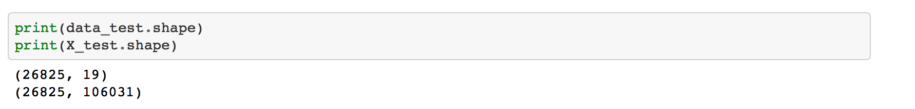
We have also transformed our X_test matrix to obtain a similar matrix, with the same number of features as X_train.
Cross Validation
After both the training and test matrices are obtained, we build a grid search pipeline using GridSearchCV to obtain an optimized version of AdaBoostClassifier, the algorithm we chose to use for our model. We chose Adaboost because by default it’s a non-linear model, and we strongly believe that due to the number of features and the number of observations in the dataset, the decision boundary will be non-linear. Adaboost is an ensemble algorithm, and so it tends to outperform other simpler algorithms, which is another reason we chose to use it.
The GridSearchCV takes some time to run, but finally outputs our optimized classifier, which has parameters: n_estimators: and learning_rate: .
# Basic cross-validation with Grid Search CV
AdaModel = AdaBoostClassifier()
parameters = {
    'n_estimators': range(50, 200, 50),
    'learning_rate': np.arange(0.01, 0.09, 0.01)
}
clf = GridSearchCV(
    AdaModel,
    parameters,
    n_jobs=-1,
    verbose=20,
    cv=KFold(2, shuffle=True),
    scoring=make_scorer(accuracy_score))
clf.fit(X_train, y_train)

y_pred = clf.predict(X_train)
print(accuracy_score(y_train, y_pred))
1.0
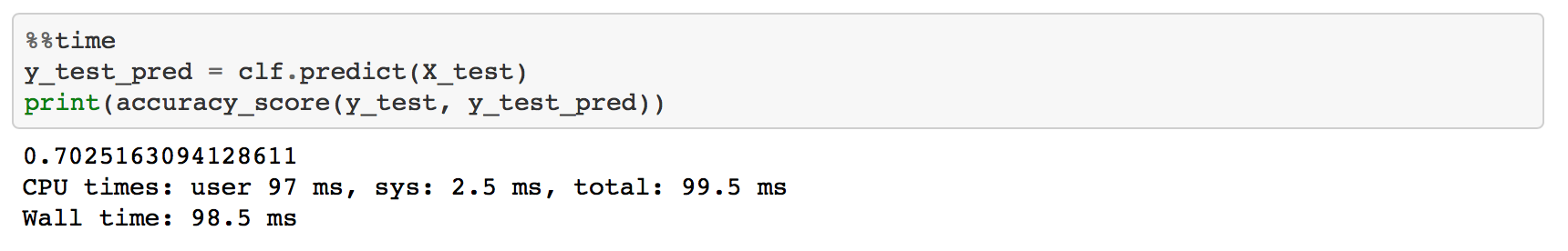
Training Results Summary
This optimized model gives us training accuracy of 1.0, and test set accuracy of .7025. On the training set, the model learns how to perfectly distinguish between tracks which should belong to a playlist and tracks which should not. On the test set, the model has about 20% higher accuracy than a random classifier would have (half of the songs in test have the target match = 1 and half have match = 0. Granted a test performance result provably better than trivial, we decided to proceed to using the AdaBoostClassifier model to actually recommend songs, and obtain an r_precision. See Model Testing and Results