Table of Contents

Project Statement and Goals
Motivation and Background
Data Description
EDA
Data Cleaning
Metrics
Model Training
Interpreting the Model
Model Testing and Results
Conclusion and What’s Next
Literature Review

Model Testing and Results

Introduction

Using the trained model, we proceed to recommend songs to our trained playlists. As mentioned, a train_test_split was done on our merged dataset to obtain an X_train and an X_test. This train_test_split was done in a stratified manner on the playlist_id feature, meaning that for every playlist in the data, 30% of songs were reserved for testing. This train_test_split strategy enabled us to simulate real world environments, where the Spotify team will have a seed playlist to start with, from which they’ll recommend songs. In the future we’d like to experiment with creating our own train-test splits rather than using the sklearn library to get more intuition on the process and a finer degree of control. See Model Training for code of the data split.

To make things run faster, we chose to predict only whether a “test set track” belonged to a particular playlist. We did not do the prediction of playlist membership on the training set tracks: our algorithm had already seen them so it will be a trivial task to predict on the tracks in the playlist in the training set. In addition, predicting on only test set tracks was also helpful in reducing computation time and quickly getting feedback on how our model performs in a track recommendation environment. In the future we would like to predict on training tracks that were not in the playlist we are currently making recommendations for.

The above caveat beside, when 2000 playlists were loaded, there were still about 26000 unique test set tracks. Our test pipeline therefore consisted of appending all of these 26000 unique test set tracks to each and every playlist trained on and predicting track membership. For the 2000 playlists, our model will need to do about 52 million predictions (26000 * 2000).

For every playlist, we predict track membershp for the 26000 test set tracks. Runtime is slow; one potential improvement could be vectorizing the pipeline rather than using a for loop.

After prediction, we ranked the tracks by probabilities of match = 1. We calculate the r_precision metric with the ground truth tracks which we reserved for training. On average, playlists have about 66 tracks, so about 20 tracks will be reserved for the testing pipeline to calculate the r_precision. The task for AdaBoost is not a trivial one: out of 26000 tracks (using 2000 playlists), can the model rank the tracks by probability, such that the ground truth tracks present in the test set (which the algorithm didn’t see before) are ranked first?

Code to test AdaBoost and Return R-Precision Score

r_precisions = []
pbar = tqdm(data_test.groupby(['playlist_pid']))
for pid, df in pbar:
    p_info = df[playlist_df.columns].iloc[0]
    labels = y_test.loc[df.index]
    
    # Positive Tracks
    positive_tracks_idx = labels[labels == 1].index
    positive_tracks = data_test.loc[positive_tracks_idx]
    sp_positive_tracks = vectorizer.transform(positive_tracks.values)
    
    # Negative Tracks
    negative_tracks_idx = ~np.isin(data_test.index, positive_tracks_idx)
    negative_tracks = data_test[negative_tracks_idx].drop(
        playlist_df.columns, axis=1)
    negative_playlist = np.array([p_info.values] * len(negative_tracks))
    negative_playlist_samples = np.hstack([negative_tracks, negative_playlist])
    sp_negative_tracks = vectorizer.transform(negative_playlist_samples)
    # from IPython.core.debugger import set_trace; set_trace()
    
    # Test Tracks
    test_tracks = vstack([sp_negative_tracks, sp_positive_tracks])
    index_order = negative_tracks.index.append(positive_tracks_idx)
    
    # Predict, r_precision
    y_prob = clf.predict_proba(test_tracks)
    # from IPython.core.debugger import set_trace; set_trace()
    y_pred = np.argsort(-y_prob[:,1])
    best_pred = index_order[y_pred]
    if len(positive_tracks_idx) > 0:
        r_precisions.append(r_precision(positive_tracks_idx, best_pred))
    pbar.set_description("{}".format(np.mean(r_precisions)))

R-Precision Results

Our mean r_precision returns at about 0.12. This means that out of 25 ground truth songs, 3 will be present in the top 25 predictions. We did some sanity checking to see how our model is doing compared to other Spotify RecSys Challenge participants and see that the best model had an r_precision of 0.224656, where they used the entire dataset.

Predictions for a Single Playlist

A function to get top 10 predictions for a particular playlist name

This function is similar to the one used for computing r-precision with the functionality to return the top 10 predictions

def get_track_predictions(playlist_name, top_tracks=10):
    """
    Function to get track predictions for a single playlist
    playlist_name should be in the form of a string.
    """
    for pid, df in pbar:
        p_info = df[playlist_df.columns].iloc[0]
        if p_info.playlist_name == playlist_name: 
            labels = y_test.loc[df.index]

            # Positive Tracks
            positive_tracks_idx = labels[labels == 1].index
            positive_tracks = data_test.loc[positive_tracks_idx]
            sp_positive_tracks = vectorizer.transform(positive_tracks.values)

            # Negative Tracks
            negative_tracks_idx = ~np.isin(data_test.index, positive_tracks_idx)
            negative_tracks = data_test[negative_tracks_idx].drop(
                playlist_df.columns, axis=1)
            negative_playlist = np.array([p_info.values] * len(negative_tracks))
            negative_playlist_samples = np.hstack([negative_tracks, negative_playlist])
            sp_negative_tracks = vectorizer.transform(negative_playlist_samples)
            # from IPython.core.debugger import set_trace; set_trace()

            # Test Tracks
            test_tracks = vstack([sp_negative_tracks, sp_positive_tracks])
            index_order = negative_tracks.index.append(positive_tracks_idx)

            # Predict, r_precision
            y_prob = AdaModel.predict_proba(test_tracks)
            # from IPython.core.debugger import set_trace; set_trace()
            y_pred = np.argsort(-y_prob[:,1])
            best_pred = index_order[y_pred]
            if len(positive_tracks_idx) > 0:
                print(r_precision(positive_tracks_idx, best_pred))
                print(data_test.loc[best_pred[:10]].loc[:,['track_artist_name','track_name']])
            break
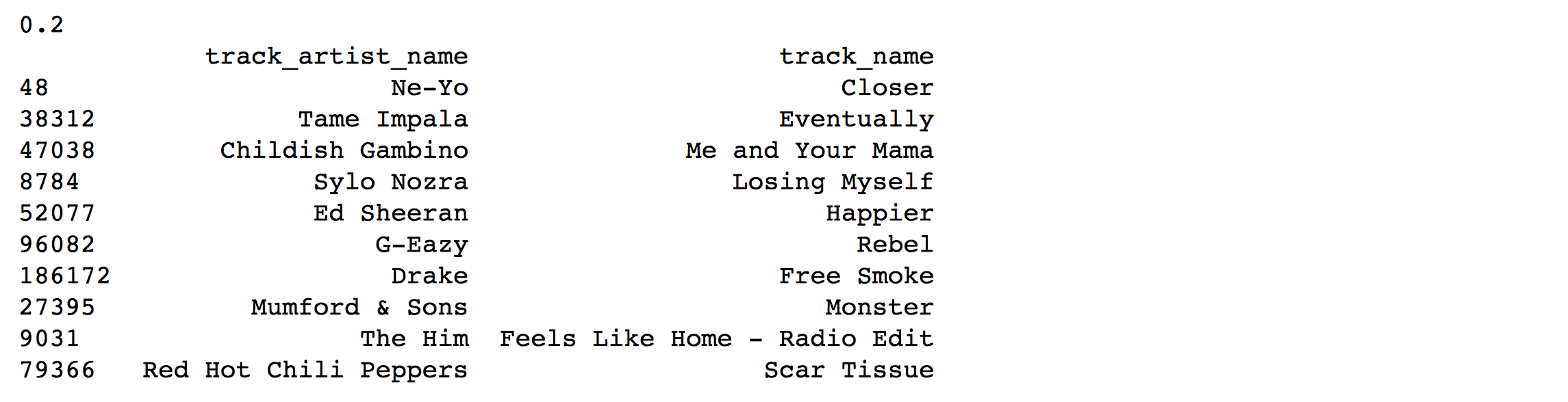
get_track_predictions('Throwbacks', top_tracks=10)

Conclusion

The predictions that we get for the playlist “throwbacks” are very reasonable! AdaBoost is suggesting songs that are popular among playlists found in MPD. The songs roughly fit the genres and moods found in “throwbacks”. Perhaps the playlist name played a role in predicting the Red Hot Chilli Peppers song ‘Scar Tissue’, a throwback to what you might have heard on the radio on the way to the beach in 1999! The song ‘Closer’ by the artist Ne-Yo that was predicted to match is a direct hit: it is in “throwbacks” in the training set.

We are excited to use our model to get suggestions for our own playlists, and we have a function that is ready for us to add playlists to the dataset in the future. See Metrics for that function.